

Introduction
This is Part 3 of a three-part series benchmarking shared_buffers behavior on a 128 GB PostgreSQL 18 system. Parts 1 and 2 examined throughput, memory behavior, and huge page utilization across TPC-B and analytics workloads. This article explores the economic tradeoffs between memory and storage, introducing metrics that help identify workload-specific configurations that minimize the cost of delivering a given level of performance.
In modern cloud environments, resource consumption is metered across multiple independent dimensions like storage IOPS, throughput, CPU time, and sometimes WAL or network egress. Cloud infrastructure pricing is often discontinuous, a modern increase in required IOPS or CPU may require utilization of a higher resource tier, often at a much higher cost. This blog is focused on the cost of providing that performance and some possible ways of optimizing the cost.
I fully acknowledge that efficiency will absolutely depend on the actual hardware being utilized, and this set of metrics is based on a hardware sample of one. This is meant as a beginning and I am more than happy to continue this experiment for any systems I may be given access to. I do intend to follow up with both the code and instructions on how these metrics can be created for other environments, if anyone wants to re-create these or similar experiments.
Normalizing Efficiency
All metrics below are expressed per million transactions (labelled mtxn) executed over 1 hour test duration. The transactions attempt to represent a relatively stable amount of work within each type of workload, although database drift due to random selection of parameters will cause some variation over test duration.
Throughout these experiments my system recorded 27.6 billion transactions, and I expect the random effects to largely average out.
The way to read these graphs is to:
- First identify whether your workload is more similar to TPC-B (single value updates accessed via index and simple, highly specific filters) or Analytics (complex queries with joins between tables).
- Identify whether your hot data fits within memory, ws_30, or ws_100 when it does not.
- Examine the range of consumption of a resource to provide the same amount of work.
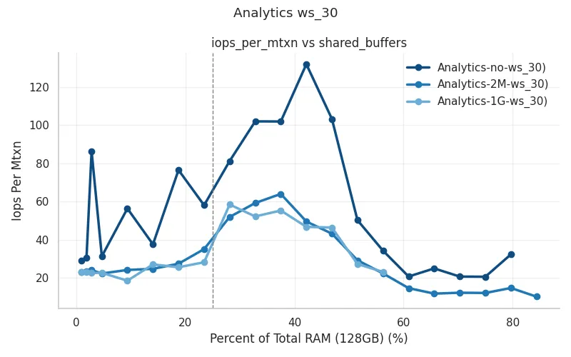
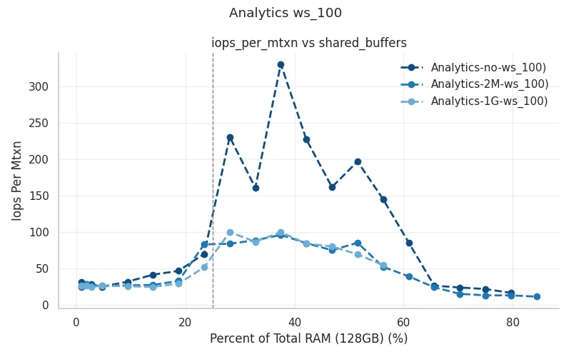
For example, for an Analytics style workload that fits in memory, the range of disk IO operations per second for the default 4kB pages ranges from 30 to 130 depending on shared_buffers allocation, representing a 5 to 6 fold difference in the rate of disk requests.
If we are trying to optimize the use of an overloaded disk, we can see that either reducing shared buffers to around 5% or increasing past 60% of total RAM should greatly reduce disk IOPS. Additionally, changing to huge_pages should allow for additional improvement.
More generally, effective memory utilization is often one of the most direct paths to better performance, but it can also be viewed as a cost tradeoff. In some environments, additional memory can reduce demand on more expensive or more constrained resources, especially disk I/O. This does not mean that maximizing memory allocation is always optimal from a cost perspective.
IOPS per Million Transactions
One of the first performance bottlenecks on a database is the disk, and a disk is often a very large component of the total cost of a cloud database. Also, hot standby environments and read replicas very frequently require identical size and specification disk as well. Differences in these graphs can be attributed to additional caching or swapping of memory, additional disk lookups when data is not available in various caches.
Definition: This is the total number of disk reads and disk writes performed by postgresql processes divided by the total time performing IO by the same processes for each experiment. This metric is an average IOPS normalized per million transactions (mtxn) for each experiment.
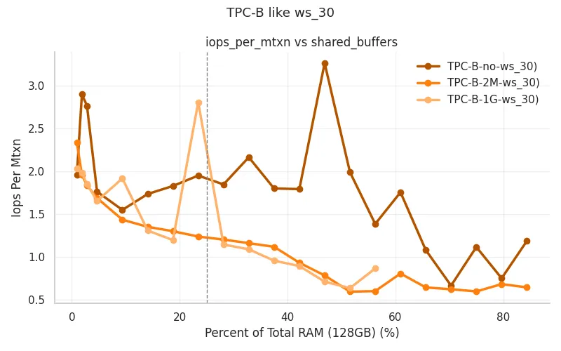
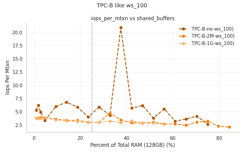
For TPC-B style workload we see that increasing shared buffers as a percentage of total RAM will decrease the IO load on the disk to provide the same unit of work. When the work does not fit in RAM, the reduction is negligible as many requests have to retrieve data from disk as it is not available in a cache.
For analytics workloads, low memory and high memory allocation utilize the disk more efficiently than setting shared_buffers between 20 and 60 percent of total RAM. When both shared_buffers and the OS file cache are similarly sized, they will likely, largely, contain a duplicate of the same data when the database is the primary consumer of that machine. That effectively halves the available memory of the system.
In both TPC-B and Analytics style workloads we can see that the default 4kB data pages come with an increased disk utilization. My theory is that this is related to the behavior identified in Part 2 of this blog. When utilizing 4kB pages, the kernel appears to move things around in order to maintain a higher than anticipated file cache.
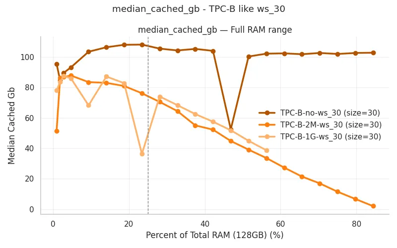
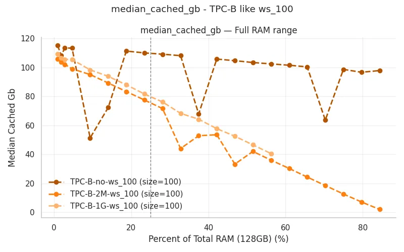
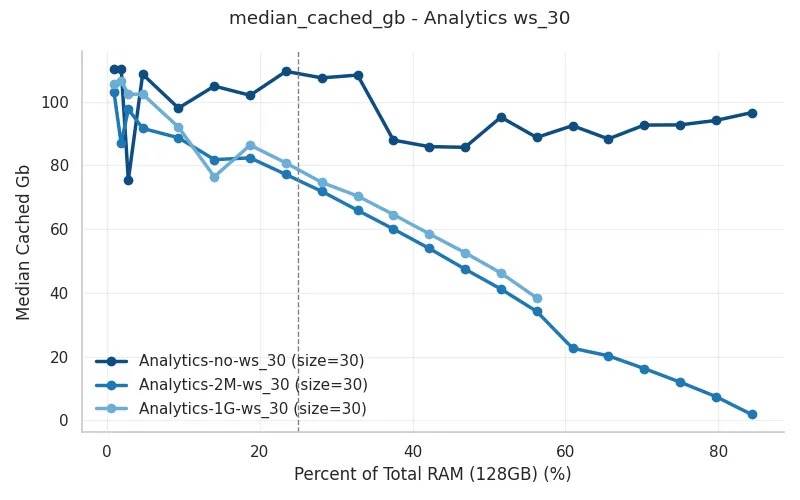
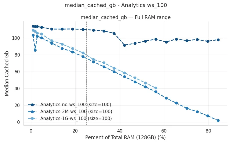
Throughput (MB/s) per Million Transactions
While IOPS measures the number of requests, the size of requests can vary as well. In some circumstances the kernel is able to combine two, or more, IO requests into a single, longer one. This metric measures an overall, average MB / second required from the disk to support one million transactions.
Definition: The average rate of disk reads and writes required for each million transactions. This metric helps distinguish between “chatty” workloads (high IOPS, low throughput) and “bulk-heavy” ones.
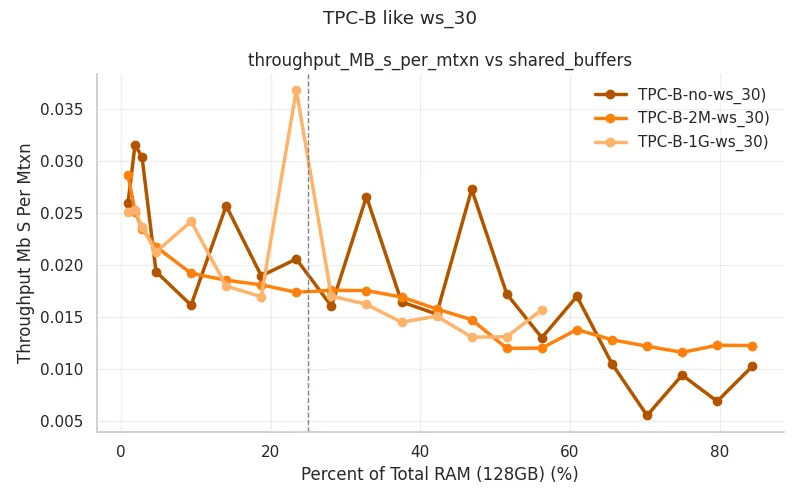
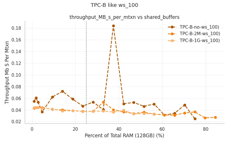
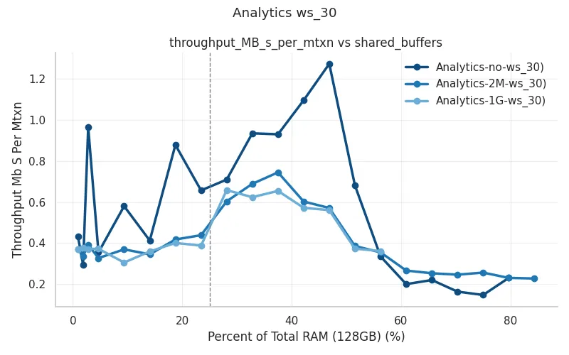
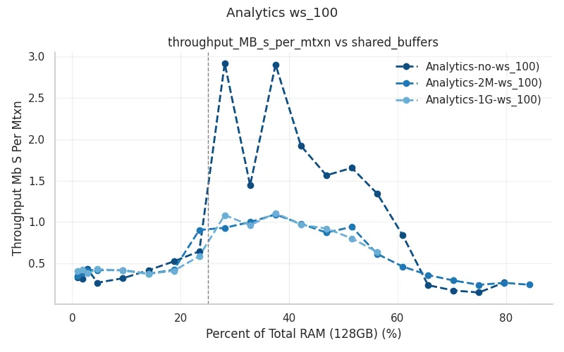
Just as before, we can see that TPC-B style workloads do not really affect the rate of disk reads and writes with changing shared_buffers. We continue to see that for Analytics workloads there is a significant average disk throughput, showing about three-fold difference between high and low when using huge_pages and over 5 fold difference when using 4kB pages.
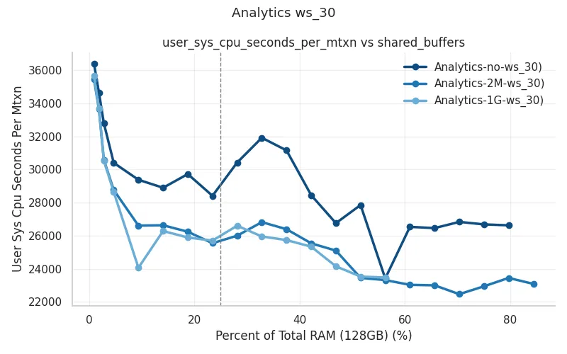
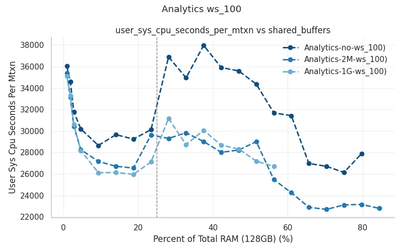
User + System CPU Seconds per Million Transactions
This metric tracks how many CPU slices postgresql processes used over each experiment, normalized to 1 million transactions. Effectively showing us how hard the CPU had to work to provide all information.
I am including both the user space and the kernel work attributed to each process, but removing any IO or network waits, as during those times the cpu would be available for other processes. Differences in these metrics could be attributed to buffer and lock management, kernel overhead, IO and memory management, context switching, etc.
Definition: For every PostgreSQL process, how much time was actually spent running on a CPU, removing any time that was spent waiting on resources like IO. This is actual execution time when the scheduler has allocated this process to a CPU and includes system CPU time on behalf of the process and is normalized per mtxn.
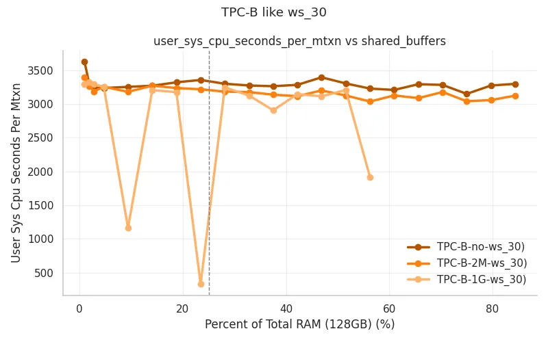
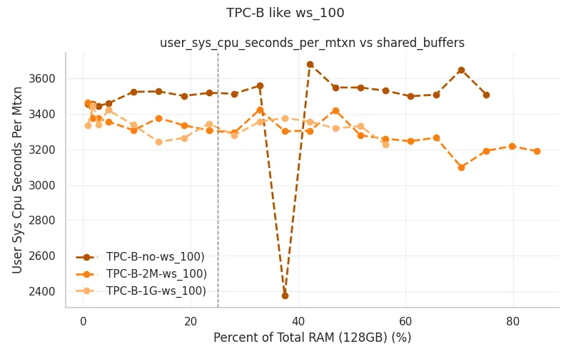
These graphs are largely stable for TPC-B style workload, with an exception of specific data points. At this point I’m inclined to treat these points as anomalies, since the value does come back to the previous level during the next sample.
Analytics style workloads show about a 50% difference in CPU usage as between low and high shared_buffers allocation.
I believe this is largely the overhead of managing small shared_buffers, and deciding which data pages to evict. Again, we see a higher CPU utilization when using the default 4kB pages, likely due to additional management and swapping being performed on by the kernel.
Non voluntary Context Switches per Million Transactions
In a Linux kernel, a process is given access to a CPU for a specific time slice. If there are additional processes ready to execute, it can be switched out for another ready to run process. That type of switch is involuntary and shows that there were more processes ready to execute than CPUs available to run them.
When a process is attempting to perform an IO operation and it knows it needs to wait, it can perform a voluntary context switch, giving up the CPU for another process that is ready to run. Non voluntary context switches represent contention for the CPU, where there is more work ready to go than there are processors available.
Definition: Average number of involuntary context switches per million transactions.
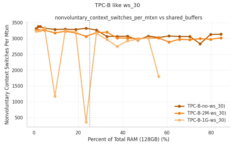
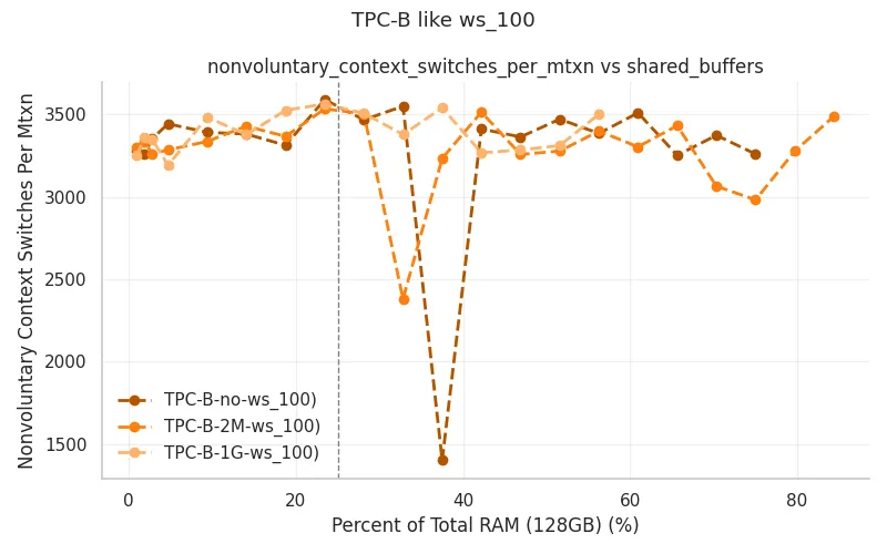
While context switching does impose a bit of overhead like reloading CPu registers and TLB caches, that overhead is very small compared to the overall CPU utilization. It does mean that many processes were ready to execute but had to wait. I would expect this behavior to show up as latency experienced by clients.
I am including this graph as an idea for a followup. My theory is that this overhead can become much more visible when using thousands of client connections, and it could be a metric to track operationally to see how it changes over time.
Interpreting These Metrics Together
In conclusion, no single metric defines efficiency and these specific graphs only include an example of a single hardware and OS configuration. The intent is to look at orders of magnitude changes between various efficiencies. Does it make sense to increase 30% CPU to reduce IOPS by 2x?
My hope is that we can use these types of graphs to shape the work being performed to the hardware capabilities and the work type.
There is also a possibility of measuring these metrics in near real time in order to detect inefficiencies or bottlenecks. After all, just because the CPU or disk is working hard, does not necessarily mean that it is doing useful work and a different configuration will not be able to achieve it more efficiently. We can optimize PostgreSQL not just for performance, but for cost efficient performance.