

Foreword
This is Part 1 of a three-part benchmark series examining shared_buffers behavior on large-memory PostgreSQL systems and how different workload patterns influence the benefits obtained from PostgreSQL’s buffer cache.
This experiment grew far beyond the original scope. What began as a straightforward benchmark with a simple graph turned into a rabbit warren of side investigations while trying to understand what the system was actually doing.
Some questions were answered. Some of those answers led to new tunnels worth exploring.
If you’ve observed similar behavior or have identified flaws in the assumptions, I would welcome the discussion.
As a result, this blog is now split into 3 parts:
- Measuring shared_buffers behavior - setup and initial results
- When should you use huge_pages in PostgreSQL? how huge_pages affects system behavior
- PostgreSQL shared_buffers and efficiency metrics - looking beyond raw performance to how efficiently work is performed
The Role of shared_buffers in Large‑Memory PostgreSQL
Shared_buffers sit at the heart of PostgreSQL’s internal cache. It stores recently accessed data pages so PostgreSQL can avoid invoking the operating system’s I/O path for cached data. By keeping hot pages in memory, PostgreSQL reduces latency, reduces disk traffic, and improves overall throughput.
The classic guidance for sizing shared_buffers dates back to PostgreSQL 8.3 (released in 2008) when a 1 GB RAM machine was considered large. Today’s large servers can hold hundreds of gigabytes or even terabytes of memory.
The best system I had available for this experiment is a 128 GB system AMD Ryzen 7 7840U, 8-core system running Ubuntu 24.04. While not an enterprise NUMA server, it still provides enough memory scale to expose behaviors that smaller 16-32 GB systems often mask.
That amount of RAM allowed testing and scaling shared_buffers values from 1 GB up to around 110 GB, while still leaving memory for the operating system.
A database system (Operating System included) needs to partition available memory into many tasks:
- OS/kernel memory: The OS needs to be able to operate effectively, the kernel and any running software requires its own memory
- Filesystem cache: filesystems need a cache to smooth out that access
- PostgreSQL shared buffers: The database needs its shared_buffers as well as
- work_mem for all active connections that are used to throw a load significant enough to properly test performance
- Background services and monitoring tools
My working theory was that balancing these tasks on a system with 16GB or 32GB of RAM is likely exposing bottlenecks. The tradeoffs become easier to observe on larger systems.
Why shared_buffers is Not Set-and-Forget
The amount of memory allocated to shared_buffers interacts directly with the workload’s characteristics. Detailed descriptions are included further down in this document.
- Working set size: This is the subset of the database that is frequently queried and modified
- Workload type: TPC-B style point lookups vs. Analytics style multi-table joins
- Huge_pages: The benefits and drawbacks of using huge_pages on large systems (Part 2)
In short, shared_buffers is not a universal setting. The overall performance of the system depends on the types of workload as well as shared_buffers allocation balancing between OS file cache and direct postgresql memory. In this series we will take a peek at some of the mechanisms that are involved.
Test Database
For this project I created a synthetic database designed to mimic a social media platform, including users, posts, messages, tags, follows and likes.
The database occupied roughly 250 GB of disk space, or about 2 times the total amount of system RAM available. Because the workloads included both read and write queries, the database size grew a bit over the test duration.
The data-generation scripts randomized user activity, message distribution, post and message lengths, and created both narrow and wide tables. This allowed for more realistic access patterns, complex joins, and a reasonable mix of supporting indexes.
A full write-up of the data creation, monitoring, and analysis process will be published separately.
Workloads
I decided to implement two distinct workloads. A TPC-B style that is similar to the default pgbench test as well as a more complex analytics style workload. If your queries are multiple lines (or pages) long, then your workload is very far from TPC-B and much closer to the Analytics style implemented here. One of my goals was to highlight how the performance changes depending on the workload.
The memory access of the two workloads is also very much different. TPC-B performs point accesses (select or update of a single row via primary key). On average, that specific data page is not likely to be needed again. Analytics workload performs joins between tables, the same data pages are accessed and modified by multiple queries, making the decision of what to keep and what to throw away far more important to the overall performance of the database.
The overall balance of memory allocation between the database (shared_buffers) and the OS (kernel cache) also plays a major role in overall performance.
- TPC-B‑style point‑update workload
- 10 % write / 90 % read ratio
- Selects and Updates target either the last 30% of rows or the full table (random ID selection)
- All tables participate, exercising shared_buffers across the whole data set
- Analytics‑type workload
- 10 % write / 90 % read ratio
- Selects and Updates target either the last 30% of the rows or the full table.
- Heavy multi‑table joins (e.g., users ↔ posts ↔ post_tags ↔ tags)
Designed to stress the buffer cache with larger (but bounded) results sets. The intent was for the amount of work to remain stable during each run, so the actual amount of work does not increase as data grows.
Working Set & Performance Impact
The working set is the portion of the database that must be residing in memory to satisfy the current workload without excessive paging. In this experiment two values were chosen:
- 30% working set – Only the most recent 30% of rows are actively accessed (simulating a “hot” slice of data). This value was selected as it should be satisfied with approximately 75 GB of RAM
- 100% working set – The entire dataset (250GB+) is subject to activity.
Between these two conditions we observe how PostgreSQL changes its behavior when the working set can no longer fit in memory and the database is forced to constantly evict and load pages from disk. The 30% working set is estimated to require approximately 75 GB of RAM, so we can also see the performance tradeoff between having either the OS file cache or PostgreSQL shared_buffers large enough to accommodate it.
Experimental Procedure (Brief Overview)
After the synthetic social‑media dataset was generated, the database was vacuumed and analyzed and statistics reset. Its data directory was then frozen as a template. Prior to every test run the PostgreSQL server was stopped, the data directory was rsynced back from this template to eliminate any lingering caches or drift, and shared_buffers (and any required kernel parameters) were adjusted to the desired values.
Data‑collection agents were then started and a one‑hour pgbench execution was launched using the selected workload (specifying working set and workload type). Between runs the system was given a few minutes to let the OS and disks settle before the next iteration.
Metrics Collected
- Full pgbench output for each experiment
- CSV snapshots of pg_stat_io, pg_stat_database, pg_stat_statements, pg_statio_user_tables, and pg_statio_user_indexes taken at the end of each run
- OS‑level statistics captured every 5 seconds (e.g., /proc/meminfo, /proc/diskstats, /proc/pressure/{cpu,memory,io})
- Per‑process PostgreSQL details collected on the same schedule (ksm_stat, io, sched, schedstat, stat, statm, status)
These measurements provide a comprehensive view of both database‑internal behavior and underlying system resource pressure throughout the benchmark. The data collection process is relatively light weight, either taking place after the experiment (CSV dumps of PostgreSQL statistics tables) or requiring a copy of the specific files from /proc filesystem. The logging process injects a timestamp for each line of log collected and performs no other processing during the experiment.
After the experiment there are parsing scripts that process each type of data and outputs them into a CSV file, calculating delta values between fields where required. Those CSV files are then imported into a duckdb database for analysis and correlation.
Results
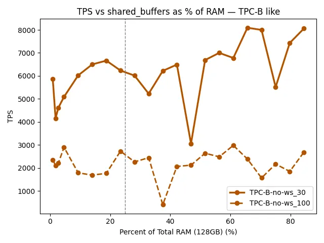
TPC-B like workload
In this point workload we can see an immediate and significant performance difference between working within the available memory vs. spilling over to disk.
The recommendation of 25% is a reasonable value, although there appear to be some benefits to giving PostgreSQL a bigger slice of system RAM when the working set does not fit in available memory. The shape of the two lines has some similarities.
I plan to revisit the dip in performance near the center of the graph in part 3 - when we look at efficiency.
The following graphs show the cumulative resource stall time recorded by Linux PSI (Pressure Stall Information). For each resource (CPU, I/O, and memory), the lines represent the total number of seconds the system experienced partial contention (“some”) and complete contention (“full”) during the run.
Because PSI totals are cumulative stall time, higher values directly indicate more time lost to contention for that specific resource. The fixed y-axis of 1 hour total experiment time, allows consistent comparison across configurations, making it easy to identify the relative overall wait for each resource.
These graphs show that the overall IO pressure was higher during the ws_100 run (as expected) and that memory access was not a significant bottleneck.
WS_30 Run
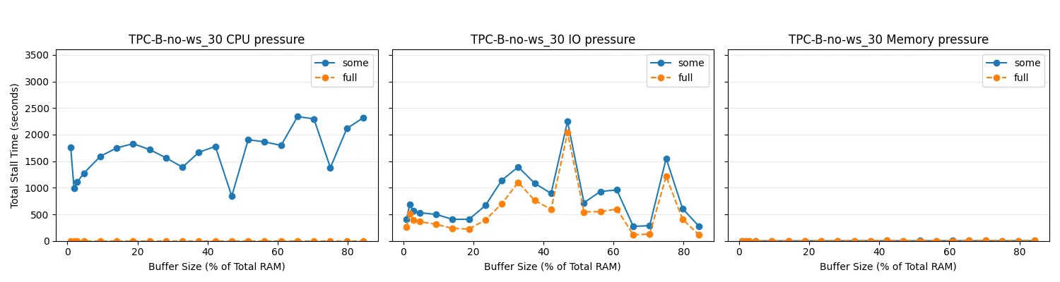
For the ws_30, we can see that IO pressure is higher between 20 and 60% of total RAM. Within this range, the entire working set is expected to fit within either the OS file cache or shared_buffers.
On the upper end, we do have some anomalous points which could be noise or an effect of continuing to move memory from OS file cache to shared_buffers that already hold the entirety of the working set.
WS_100 Run
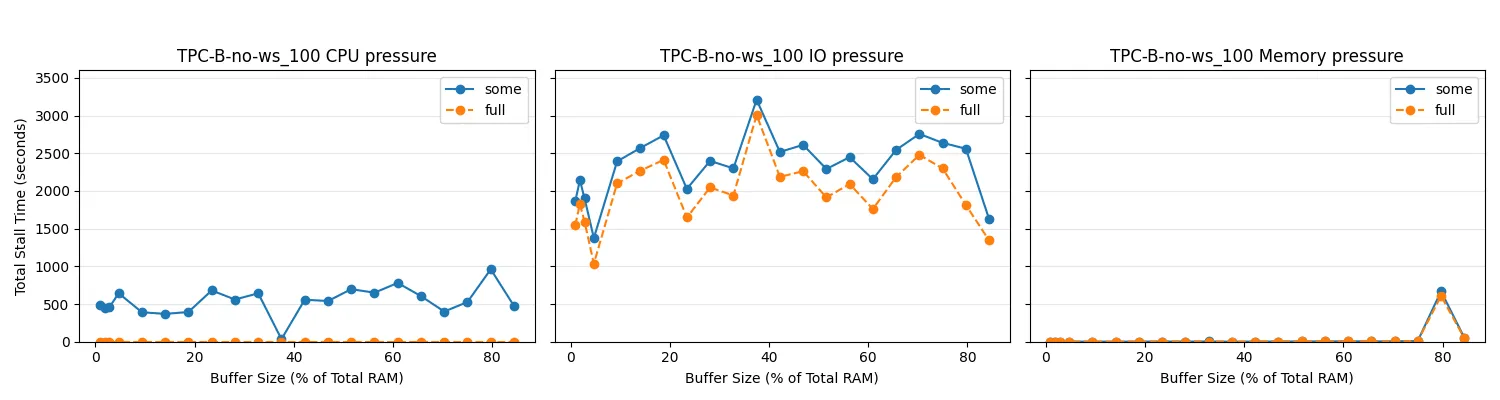
On the upper end, we do have some anomalous points which could be noise or an effect of continuing to move memory from OS file cache to shared_buffers that already hold the entirety of the working set.
Results - Analytics workload
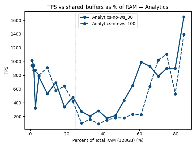
With a more complex query and pattern of memory accesses, the graphs look quite different. There is an overall performance gain from having enough memory allocated to the working set in either the OS file cache or the shared_buffers (at both ends of the range).
At the lower end (shared_buffers less than 5%), the database will store the most critical buffers and reusable information while allowing the remainder of the memory for efficient disk caching. Up until about 80% of RAM being allocated to the shared_buffers, the two strategies result in very similar performance.
At an extremely high end (approaching 90% allocation to shared_buffers), I did get a pretty significant performance increase, although I should caution that the danger of OOM is quite high and these data points had to be re-run to get usable results.
In either case, we see that the recommended 25% of shared_buffers is far from either peak for this type of workload. At that state the same data is often duplicated in both caches making that memory far less effective and reducing the overall amount of memory available.
The winning strategy appears to be maximizing the amount of data that is cached from the database. Splitting the memory between both buffers reduces the effective memory available for caching.
Looking at the Pressure Stall Information, we see that IO access was dominating the wait time, as a lot more data had to be examined to provide results to our queries. The pattern of increased disk pressure in the middle portion of the graph is still there, although we have a lot more noise at the lower end of ws_30.
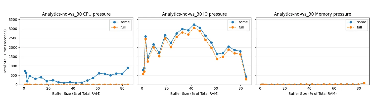
Pressure Stall Information for Analytics workload with 30% working set.
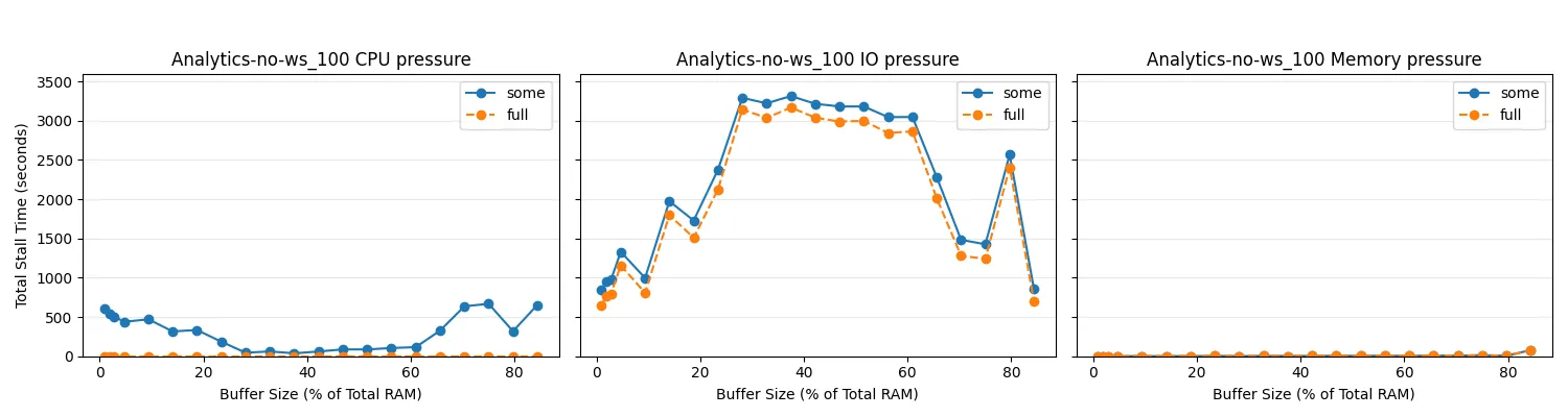
Pressure Stall Information for Analytics workload with 100% working set.
Conclusion
We are seeing significantly different behavior between the TPC-B style and Analytics workloads. It appears that more complex workloads benefit from being able to store the entire working set within a single buffer (either OS file cache or the shared_buffers).
The lowest overall performance appears to be within a range of 30 - 50% of total memory allocation to shared_buffers (for analytics style workload). There was also between 5 times and 8 times improvement in performance between the low points and either very small or very high allocation.
For the TPC-B style workload, the difference is significantly less impactful. There is about 30% improvement by allocating nearly all system memory to shared_buffers when the hot pages can fit in RAM, and negligible difference when the hot pages are larger than the system RAM. There are also areas where the performance drops which require further investigation.
Additionally, there may be some benefits to looking at linux pressure stall information to determine whether the database is largely constrained by CPU, I/O or RAM access.
We will look at this a bit more closely in part 2 and 3 of this blog, with the next part focused on utilizing huge_pages for our large shared_buffer and what benefits and drawbacks this choice may have.